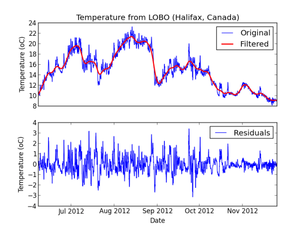
Here we apply a low-pass filter to temperature from the Satlantic LOBO ocean observatory moored in the North West Arm (Halifax, Nova Scotia, Canada).

First, we download temperature data from the LOBO buoy. The Code to do that was originally posted HERE. However, for convenience, below it is shown a shortened version of the code (note that in this instance we further converted the temperature data into a numpy array, which is required by the filtering function).

import urllib2
import StringIO
import csv
import numpy as np
from datetime import datetime

startdate = '20111118'
enddate   = '20121125'

# Read data from LOBO buoy
response = urllib2.urlopen('http://lobo.satlantic.com/cgi-data/nph-data.cgi?min_date='
                           +startdate+'&max_date='+enddate+'&y=temperature')

data = StringIO.StringIO(response.read())

r = csv.DictReader(data,
                   dialect=csv.Sniffer().sniff(data.read(1000)))
data.seek(0)

# Break the file into two lists
date, temp = [],[]
date, temp = zip(*[(datetime.strptime(x['date [AST]'], "%Y-%m-%d %H:%M:%S"), \
                 x['temperature [C]']) for x in r if x['temperature [C]'] is not None])

# temp needs to be converted from a "list" into a numpy array...
temp = np.array(temp)
temp = temp.astype(np.float) #...of floats

Now that we have data… we can proceed to design and apply the filter and make the plots…

import scipy.signal as signal
import matplotlib.pyplot as plt

# First, design the Buterworth filter
N  = 2    # Filter order
Wn = 0.01 # Cutoff frequency
B, A = signal.butter(N, Wn, output='ba')

# Second, apply the filter
tempf = signal.filtfilt(B,A, temp)

# Make plots
fig = plt.figure()
ax1 = fig.add_subplot(211)
plt.plot(date,temp, 'b-')
plt.plot(date,tempf, 'r-',linewidth=2)
plt.ylabel("Temperature (oC)")
plt.legend(['Original','Filtered'])
plt.title("Temperature from LOBO (Halifax, Canada)")
ax1.axes.get_xaxis().set_visible(False)

ax1 = fig.add_subplot(212)
plt.plot(date,temp-tempf, 'b-')
plt.ylabel("Temperature (oC)")
plt.xlabel("Date")
plt.legend(['Residuals'])

For more information, check the SCIPY Signal processing library.