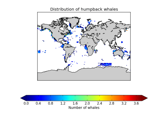
Here we download and plot “humpback whale sightings” from the OBIS SEAMAP database.

First, download the data as a .csv file. Then use following code:

import csv
import numpy as np
from mpl_toolkits.basemap import Basemap
import matplotlib.pyplot as plt

# Open file
f = open('species_180530_points.csv', 'r')

# Read file
r = csv.DictReader(f)

# Initialize empty variables
lat, lon, num = [],[],[]

# Loop to parse data into our variables
errors = 0
for row in r:
    try: # The "Try/except" routine, prevents the loop to break if there is an empty field
        lat.append(float(row['latitude']))
        lon.append(float(row['longitude']))
        if not row['count'] == '':
            num.append(float(row['count']))
        else:
            num.append(1) # If "count" is empty, replace it with a 1
    except ValueError:
        errors = errors + 1 # Simple error counter

# Set up projection and limits
m1 = Basemap(projection='mill',llcrnrlat=-90,urcrnrlat=90,\
            llcrnrlon=-180,urcrnrlon=180,resolution='c')

# Given the projection, estimate plot coordinates from lats and lons
x,y = m1(lon, lat)

# Project data points into a grid
nbins = 200
H, xedges, yedges = np.histogram2d(x,y,bins=nbins,weights=num)

# Rotate and flip H...
H = np.rot90(H)
H = np.flipud(H)

# Mask zeros
Hmasked = np.ma.masked_where(H==0,H)

# Log H for better display
Hmasked = np.log10(Hmasked)

# Make map
fig1 = plt.figure()
cs = m1.pcolor(xedges,yedges,Hmasked,shading='flat')
m1.drawcoastlines()
m1.fillcontinents()
m1.drawmapboundary()
plt.title('Distribution of humpback whales')
cbar = plt.colorbar(orientation='horizontal', extend='both')
cbar.ax.set_xlabel('Number of whales')