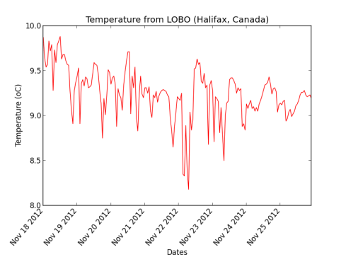
The Satlantic LOBO is a ocean observatory moored in the North West Arm (Halifax, Nova Scotia, Canada). In this post, we’ll query the LOBO server to create a temperature plot.
# First, specify the start and end dates for the query
startdate = '20121118'
enddate   = '20121125'

# Read data from LOBO
import urllib2
response = urllib2.urlopen('http://lobo.satlantic.com/cgi-data/nph-data.cgi?min_date='
                           +startdate+'&max_date='+enddate+'&y=temperature')
data = response.read()

# We use StringIO to convert data into a StringIO object
# Learn more: http://docs.python.org/2/library/stringio.html
import StringIO
data = StringIO.StringIO(data)

# read the StringIO object as it was a file
import csv
r = csv.DictReader(data,
                   dialect=csv.Sniffer().sniff(data.read(1000)))
data.seek(0)

# Break the file into two lists
date, temp = [],[]
for row in r:
    date.append(row['date [AST]'])
    temp.append(row['temperature [C]'])

# Change the time strings into datetime objects
from datetime import datetime
DAT = []
for row in date:
    DAT.append(datetime.strptime(row,"%Y-%m-%d %H:%M:%S"))

# Plot the output
import matplotlib.pyplot as plt
fig, ax =plt.subplots(1)
ax.plot_date(DAT, temp, 'r-')
fig.autofmt_xdate(rotation=50)
plt.title("Temperature from LOBO (Halifax, Canada)")
plt.ylabel("Temperature (oC)")
plt.xlabel("Dates")
plt.show()


For grabbing the data lists, r[‘temp..’] and r[‘date..’] should already be everything you need date and temp to be. You can save yourself a list traversal that way. Another time-saver would be to just map r[‘temp’] to the datetime converter and pass the list of datetimes to pyplot. It knows how to label axes given a datetime object. You can even customize the date formats based on the total length of the time period, so that short times show minutes:seconds and longer time periods don’t worry about the finer timescales.
this should replace lines 24 – 32