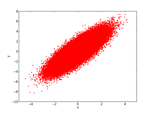
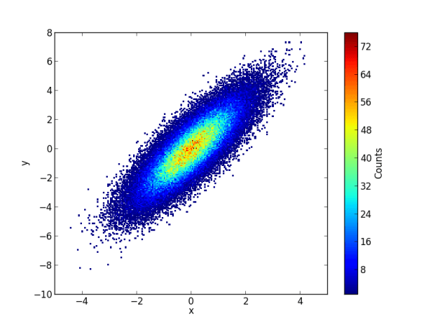
Sometimes there is too much data in a scatter plot. Therefore, it is hard to see if there are “points over points”. In this case, 2D histograms are very useful.

Raw data

2D histogram

import numpy as np
import matplotlib.pyplot as plt

# Create some random numbers
n = 100000
x = np.random.randn(n)
y = (1.5 * x) + np.random.randn(n)

# Plot data
fig1 = plt.figure()
plt.plot(x,y,'.r')
plt.xlabel('x')
plt.ylabel('y')

# Estimate the 2D histogram
nbins = 200
H, xedges, yedges = np.histogram2d(x,y,bins=nbins)

# H needs to be rotated and flipped
H = np.rot90(H)
H = np.flipud(H)

# Mask zeros
Hmasked = np.ma.masked_where(H==0,H) # Mask pixels with a value of zero

# Plot 2D histogram using pcolor
fig2 = plt.figure()
plt.pcolormesh(xedges,yedges,Hmasked)
plt.xlabel('x')
plt.ylabel('y')
cbar = plt.colorbar()
cbar.ax.set_ylabel('Counts')

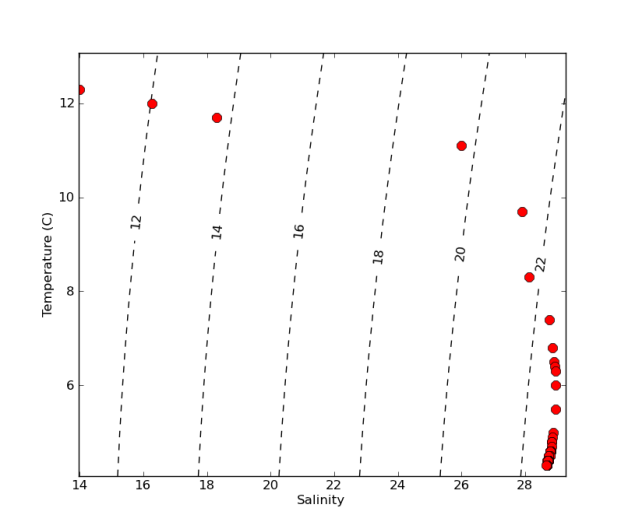
Make a temperature-salinity (TS) diagram from a CTD profile. TS diagrams show density isolines as reference and are useful to identify different water masses.

This example follows the simple tutorial on how to Plot a CTD profile… and uses the same CTD_profile.csv file.

This tutorial needs the Python Seawater Package (download HERE, or see documentation HERE).

import numpy as np
import seawater.gibbs as gsw
import matplotlib.pyplot as plt

# Extract data from file *********************************
f = open('CTD_profile.csv', 'r')
data = np.genfromtxt(f, delimiter=',')
f.close()

# Create variables with user-friendly names
temp  = data[1:,1]
salt  = data[1:,2]
del(data) # delete "data"... to keep things clean

# Figure out boudaries (mins and maxs)
smin = salt.min() - (0.01 * salt.min())
smax = salt.max() + (0.01 * salt.max())
tmin = temp.min() - (0.1 * temp.max())
tmax = temp.max() + (0.1 * temp.max())

# Calculate how many gridcells we need in the x and y dimensions
xdim = round((smax-smin)/0.1+1,0)
ydim = round((tmax-tmin)+1,0)

# Create empty grid of zeros
dens = np.zeros((ydim,xdim))

# Create temp and salt vectors of appropiate dimensions
ti = np.linspace(1,ydim-1,ydim)+tmin
si = np.linspace(1,xdim-1,xdim)*0.1+smin

# Loop to fill in grid with densities
for j in range(0,int(ydim)):
    for i in range(0, int(xdim)):
        dens[j,i]=gsw.rho(si[i],ti[j],0)

# Substract 1000 to convert to sigma-t
dens = dens - 1000

# Plot data ***********************************************
fig1 = plt.figure()
ax1 = fig1.add_subplot(111)
CS = plt.contour(si,ti,dens, linestyles='dashed', colors='k')
plt.clabel(CS, fontsize=12, inline=1, fmt='%1.0f') # Label every second level

ax1.plot(salt,temp,'or',markersize=9)

ax1.set_xlabel('Salinity')
ax1.set_ylabel('Temperature (C)')

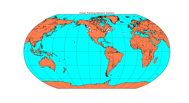
This script (contributed by Robert Branton) shows how to make a map showing the station locations of the Ocean Tracking Network (OTN).

# -*- coding: utf-8 -*-
"""
Created on Sat Feb 16 19:29:10 2013

@author: bob.branton@dal.ca

Purpose: draw simple map of Ocean Tracking Network (OTN) station locations
1) Create function to get station locations from genric node
2) Run function to get data from otn and post nodes
3) Draw empty basemap of the world
4) Overlay station locations on basemap

For more on OTN: http://members.oceantrack.org/data

"""

import numpy as np
import urllib2
import StringIO
import csv
from mpl_toolkits.basemap import Basemap
import matplotlib.pyplot as plt

#define data variable
lats, lons = [],[]

# 1) Create function to get data from otn a network node
def getdata(node):
    response = urllib2.urlopen('http://global.oceantrack.org:8080/geoserver/wfs?request=getfeature&service=wfs&version=1.1.0&outputFormat=CSV&typename='+node+':stations')
    data = response.read()
    data = StringIO.StringIO(data)
    r = csv.DictReader(data, dialect=csv.Sniffer().sniff(data.read(10000)))
    data.seek(0)
    for row in r:
        lats.append(float(row['latitude']))
        lons.append(float(row['longitude']))

# 2) Run fuction to get date from each otn node, that is otn and post
getdata('otn')
getdata('post')

# 3) Draw gloabal basemap
# map = Basemap(projection='ortho', lat_0=50, lon_0=-100, resolution='l', area_thresh=1000.0)
map = Basemap(projection='robin', lat_0=0, lon_0=-100, resolution='l', area_thresh=1000.0)
map.drawcoastlines()
map.drawcountries()
map.fillcontinents(color='coral',lake_color='aqua')
map.drawmapboundary(fill_color='aqua')
map.drawmeridians(np.arange(0, 360, 30))
map.drawparallels(np.arange(-90, 90, 30))
plt.title("Ocean Tracking Network Stations")

# 4) Overlay station locations on basemap
x,y = map(lons, lats)
map.plot(x, y, 'wo',markersize=8)
plt.show()

# done

Here we import data from a .csv file containing data from a CTD profiler (depth, temperature, salinity and fluorescence).

1. First, download the CTD_profile.csv file, and put it in your working directory.

2. Import file…

# Extract data from file *********************************
import numpy as np

f = open('CTD_profile.csv', 'r')
data = np.genfromtxt(f, delimiter=',')
f.close()

3. Create variables

# Create variables with user-friendly names
depth = data[:,0]
temp  = data[:,1]
salt  = data[:,2]
fluo  = data[:,3]
del(data) # delete "data"... to keep things clean

4. Simple plot

# Plot data ***********************************************
import matplotlib.pyplot as plt
fig1 = plt.figure()
ax1 = fig1.add_subplot(111)
ax1.plot(temp,depth,'o-')

# Draw x label
ax1.set_xlabel('Temperature (C)')
ax1.xaxis.set_label_position('top') # this moves the label to the top
ax1.xaxis.set_ticks_position('top') # this moves the ticks to the top
#ax1.xaxis.tick_top() # ANOTHER way to move the ticks to the top

# Draw y label
ax1.set_ylabel('Depth (m)')
ax1.set_ylim(ax1.get_ylim()[::-1]) #this reverses the yaxis (i.e. deep at the bottom)

plt.show()

5. More complex plot with subplots

# Three-panel plot
fig2, (ax2, ax3, ax4) = plt.subplots(1,3,sharey=True)
# Temperature
ax2.plot(temp,depth,'o-')
ax2.set_ylabel('Depth (m)')
ax2.set_ylim(ax2.get_ylim()[::-1]) #this reverses the yaxis (i.e. deep at the bottom)
ax2.set_xlabel('Temperature (C)')
ax2.xaxis.set_label_position('top') # this moves the label to the top
ax2.xaxis.set_ticks_position('top') # this moves the ticks to the top
# Salinity
ax3.plot(salt,depth,'o-r')
ax3.set_xlabel('Salinity')
ax3.xaxis.set_label_position('top') # this moves the label to the top
ax3.xaxis.set_ticks_position('top') # this moves the ticks to the top
ax3.yaxis.set_visible(False) # This erases the y ticks
# Fluorescence
ax4.plot(fluo,depth,'o-g')
ax4.set_xlabel('Flourescence (V)')
ax4.xaxis.set_label_position('top') # this moves the label to the top
ax4.xaxis.set_ticks_position('top') # this moves the ticks to the top
ax4.yaxis.set_visible(False) # This erases the y ticks

Python is a programming language that is…

• FREE! | Python operates under an open source license that makes it freely usable and distributable, even for commercial use.
• Designed for fast development | Python is an interpreted language that allows you to run code without having to compile it first. This saves time!
• General purpose |  Unlike languages that were originally developed for a specific purpose, like statistics (R) or matrix manipulation (Matlab), and then were later expanded to tackle other problems (i.e. specific-to-general approach)… Python started as a general purpose language, therefore it has been used to develop a VERY wide array of specific-purpose applications or packages.
• Runs everywhere | Windows, MAC, Linux and other.

Python was developed in 1990 by Guido van Rossum (used to work for Google, now he works for Dropbox).

You can learn more about Python in:

• Python.org
• Wikipedia
• Google’s Python class

• If you tried to open you data file in MS Excel and you got a message saying “Excel cannot open files with more than 30,000,000 rows”… you need to learn programming.
• If your expensive GIS software lacks a “button” or a tool to do exactly what you need to do… you need to learn programming.
• If you spent more than 10 hours doing monotonous copy-pastes or drag-n-drops in your favourite spread sheet… and you figure you have another 100 hours to go… you may want to conciser to learn programming.
• If you need to do the same graph or the same calculations more than a dozen times… you may want to conciser to learn programming.

“Button-based” software vs. “programming-based” software. Programs that provide “buttons” or a Graphical User Interface (GUI) are easier to figure out on your own. However, they are very limiting… that is, if there’s no “button” to do what you need, you simply cannot do it. As a rule of thumb, tasks that a LOT of people need to do, often motivate programmers to develop a “button-based” program to perform such tasks. However, tasks that only some odd ones need to do (e.g. scientists) are not enough to motivate the development of GUI-based programs, or if they do, the resulting GUI-programs are VERY expensive.

Ocean- and marine-scientists are often working at the edge of knowledge, trying to discover the unknown by means of new an innovative tools and techniques. Therefore these scientist often need to do analyses or graphs that can only be done using programming-based software. If so, their choices are (1) learn a programming language themselves, or (2) hire a student or a research assistant that knows programming. THEREFORE, students that know a programming language are more employable than students who don’t…. and that alone is a good reason why to keep reading.

If you decided to go ahead and learn a programming language, the next step is to figure out which programming language to learn?

Answer: If you are a new student starting your MSc or PhD… you may want to learn whatever programming language your fellow (more senior) students already know. Having a “buddy” programmer is key. However, if you are not tied to any language, you may want to learn a free (i.e. open source) programming language. Check R and, of course, python.

For a simple MS Excel file (file.xls) with two columns of data and the first row as headers…

Use xlrd package to read file:

import xlrd
wb = xlrd.open_workbook('file.xls')
sh = wb.sheet_by_index(0)
colA = sh.col_values(0) # Make column 1 into a Python list
colB = sh.col_values(1) # Make column 2 into a Python list
colA.pop(0) # Delete 1st row (header)
colB.pop(0) # Delete 1st row (header)
plot(colA,colB,'o')

Dependencies: xlrd

Note 1: You can import sheets by name (rather by than by_index)

wb.sheet_names() # Use this to query the sheet names
sh = wb.sheet_by_name(u'Sheet1') # Use this to load the desired sheet

Note 2: Method pop is an easy way to “pop” a element out of a list. See documentation

Useful Links:

• xlrd documentation

For a simple file (file.txt)…

colA,colB
324,234
346,341
147,346
234,567
368,405
344,643
235,235
236,567

Method 1: Open the whole file as one big string.

f = open('file.txt', 'r') # 'r' = read
lines = f.read()
print lines,
f.close()

Alternatively, file can be read into a numpy array for easy plotting

import numpy as np
f = open('file.txt', 'r')
data = np.genfromtxt(f, delimiter=',')
delete(data,0,0) # Erases the first row (i.e. the header)
plot(data[:,0],data[:,1],'o')
f.close()

Method 2: Open the whole file at once as a list of lines (i.e. each element in list = one line of the file).

f = open('file.txt', 'r') # 'r' = read
lines = f.readlines()
print lines,
f.close()

Method 3: Open a file “line-by-line”. This method doesn’t use a lot of memory (one line’s worth of memory at any given time), so it is good for really large files.

f = open('file.txt', 'r') # 'r' = read
for line in f:
  print line, # note, coma erases the "cartridge return"
f.close()